Thinking in Pallas - Sharded MatMuls
Street Fighting Kernels for TPUs
 Writing your first Pallas kernel
Express Yourself
The Pallas API is relatively small. In exchange for that limited surface area, you the developer are responsible for keeping a lot in your head. Managing different memory spaces, data hazards, synchronization, etc. Intimacy with the execution model helps us to imagine what should happen, but coaxing the provided constructs into a nicely composed, efficient kernel requires practice and patience. A reverence for stubbed toes is a prerequisite. The API is clean, but once you’re off the garden path it’s you, the hot sun, and a pile of FLOPs. Playing with Pallas kernels is an excellent way to appreciate Jax in that respect. Here we will use a distributed matrix multiply as a lens into the TPU.
GEMMs are exactly in the crosshairs of XLA, which means there is a lot we can learn from the time spent optimizing this code path. We’ll examine a matrix multiply distributed over 4 devices with an awkward partitioning scheme. In a later post we’ll extend this to larger topologies. Pallas rewards playing in the sand. I think the strangeness of this simple case gives us plenty of castles to build and knock over. You can find the code here.
If you haven’t read the Pallas docs, they provide a series of rich examples. If you’re more interested in jumping to implementations of attention, you can find them all over: paged attention, splash attention, grouped matmuls, tokamax, maxtext, and an implementation of DeepSeek’s NSA [12]. Here we focus on the simple and the small. Learning Pallas is learning to keep a small collection of primitives playing in rhythm. By allowing ourselves to play with a single problem for long enough these mechanisms start to snap together.
Set Up
The code to generate the matrix multiply we’ll be analyzing looks as follows:
import jax
import jax.numpy as jnp
from jax.sharding import NamedSharding, PartitionSpec as P

m, k, n = 16384, 16384, 8192
k1, k2 = jax.random.split(jax.random.key(0), 2)
lhs = jax.random.normal(k1, (m, k), dtype=jnp.bfloat16)
rhs = jax.random.normal(k2, (k, n), dtype=jnp.bfloat16)

mesh = jax.make_mesh((2, 2), ('x', 'y'))
lhs_sharding = NamedSharding(mesh, P('x', 'y'))
rhs_sharding = NamedSharding(mesh, P('x', None))
o_sharding = NamedSharding(mesh, P('x', None))
We have two matrices – one lhs matrix with dimensions [16384, 16384] and one rhs matrix with dimensions [16384, 8192] – that require 512 MiB and 256 MiB of HBM, respectively, in bf16. We are running on 4 TPU v5e, sharding the arrays over a 2x2 mesh of devices with dimensions x and y. Borrowing the named-axis notation conventions found in [3], we want to compute the following matmul:
The total FLOPs we need to perform this operation are 2*M*K*N = 4.4 TFLOPs and the arithmetic intensity on a single device is $\frac{2 \cdot M \cdot K \cdot N}{2 \cdot MK + 2 \cdot KN + 2 \cdot MN}$ = 4096 FLOPs/byte. The arithmetic intensity roofline magic number on TPUv5e is 240 [2], so this is a compute-bound operation on a single device. If you’re coming from [3], there’s a discussion in the comments about how the authors visually represent the partitioned arrays. I too fell victim to this waffling, so it’s worth stepping through. We’ll lean on jax.debug.visualize_array_sharding to double check where data gets assigned. These visualizations are from the perspective of the global array(s). We interpret this as saying region I of the global array is located on TPU J. It’s tempting to assume that it also conveys information about the physical layout of devices, but that’s where we need to be cautious. The devices are grouped into pairs, but the coordinates of the devices diverge from the implicit information communicated by the debug visualizations. We can confirm that the data on each device matches the debug visualization. Devices 0 and 1 own the top half of our dimension M, [0, 8192], and partition the columns of dimension K into [0, 8192] and [8192, 16384]. Devices 2 and 3 own the bottom half of dimension M, [8192, 16384], and partition the K dimension similarly. The same can be shown for our rhs matrix. From the perspective of our mesh, x partitions run north-south, and y partitions run east-west. Our debug visualization was correct, with respect to the device mesh. If we were to instead consider the physical coordinates of our devices, then our interpretation would be different. In that coordinate system, TPUs are z-ordered along columns, so Devices 0/1 and Devices 2/3 are North/South neighbors. We would instead say that our x partition of K runs east-west. We rely on Jax to handle the plumbing. When in doubt, lean on the debug visualization to be your guide.A note on sharded arrays
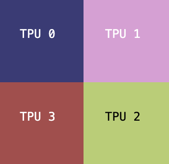 Our LHS matrix
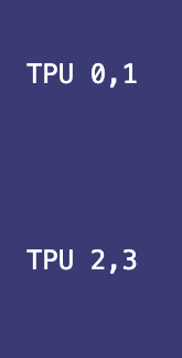 Our RHS matrix
> mesh.devices

array([[TpuDevice(id=0, process_index=0, coords=(0,0,0), core_on_chip=0),
        TpuDevice(id=1, process_index=0, coords=(1,0,0), core_on_chip=0)],
       [TpuDevice(id=3, process_index=0, coords=(1,1,0), core_on_chip=0),
        TpuDevice(id=2, process_index=0, coords=(0,1,0), core_on_chip=0)]],
      dtype=object)
> for i in lhs.addressable_shards:
>     dev = i.device
>     idx = i.index
>     print(f"Device:{dev}\nID:{idx}")

Device:TPU_0(process=0,(0,0,0,0))
ID:(slice(0, 8192, None), slice(0, 8192, None))
Device:TPU_1(process=0,(1,0,0,0))
ID:(slice(0, 8192, None), slice(8192, 16384, None))
Device:TPU_3(process=0,(1,1,0,0))
ID:(slice(8192, 16384, None), slice(0, 8192, None))
Device:TPU_2(process=0,(0,1,0,0))
ID:(slice(8192, 16384, None), slice(8192, 16384, None))
> for i in rhs.addressable_shards:
>     dev = i.device
>     idx = i.index
>     print(f"Device:{dev}\nID:{idx}")

Device:TPU_0(process=0,(0,0,0,0))
ID:(slice(0, 8192, None), slice(None, None, None))
Device:TPU_1(process=0,(1,0,0,0))
ID:(slice(0, 8192, None), slice(None, None, None))
Device:TPU_3(process=0,(1,1,0,0))
ID:(slice(8192, 16384, None), slice(None, None, None))
Device:TPU_2(process=0,(0,1,0,0))
ID:(slice(8192, 16384, None), slice(None, None, None))

Each device holds one 128 MiB quadrant of lhs and a 128 MiB row stripe of rhs, quartering the per-device FLOPs from 4.4 TFLOPs to 1.1 TFLOPs. If we assume the same idealized data access pattern as in the single-device case, the local arithmetic intensity is ∼2731 FLOPs/byte, still compute bound, but the wrinkle is in the contracting dimension. Lhs is partitioned over y and rhs over x, splitting K over different mesh dimensions.

Imagine we want to compute the above product. We first rotate the colored K-stripes of lhs so they align with the contracting dimension of rhs. For a given lhs stripe, we sweep across the output width N, multiplying against each rhs tile in turn and writing the corresponding output tiles. Once we’ve traversed the full range of N for that lhs stripe, we advance to the next lhs stripe and repeat.

Comparing the data local to Devices 0 and 1 we see that Device 0 has corresponding lhs and rhs data, but Device 1 does not. That mismatch means not every device holds the data it needs to immediately begin useful work, so communication is required before the computation can fully proceed. This is a great reference tool to help build intuition for sharding data over devices.

This mismatch becomes more pronounced as the topology grows. Only the on-diagonal devices begin with matching lhs and rhs shards. The off-diagonal devices cannot begin computing their portion of the GEMM. In an NxN mesh, the percentage of devices that initially stall without collectives for this partitioning scheme grows as 1 - (1/N). The communication burden scales with larger topologies.
The shorthand from [3] is excellent for quickly mapping named-axis notation to collectives. In summary:
- All Gather removes a subscript from a sharding, gathering the shards
- $AllGather_{X}[I, J_{X}] \rightarrow A[I, J]$
- All Reduce removes an “un-reduced” suffix, leaving the array unsharded along that axis
- $A[I, J_{X}] \cdot_{LOCAL} B[J_{X}, K] \rightarrow C[I, K]\{U_{X}\}$
- $AllReduce_{X}C[I, K]\{U_{X}\} \rightarrow C[I, K]$
- Reduce Scatter removes an “un-reduced” suffix from an array by summing shards over that axis, leaving the array sharded over a second axis
- $[A_{X}, B]\{U_{Y}\} \rightarrow [A_{X}, B]$
- All to All moves a subscript from one axis to another, resharding the axes
- $[A, B_{X}] \rightarrow [A_{X}, B]$
Below you can experiment with all-gather and all-to-all collectives to change the data placement on each of our devices. Rotate the lhs matrix to see when shards of data between the two matrices are aligned.
Baseline Jax Matmul
Simple GEMM
def jax_matmul(lhs: jax.Array, rhs: jax.Array) -> jax.Array:
    return jnp.matmul(lhs, rhs)
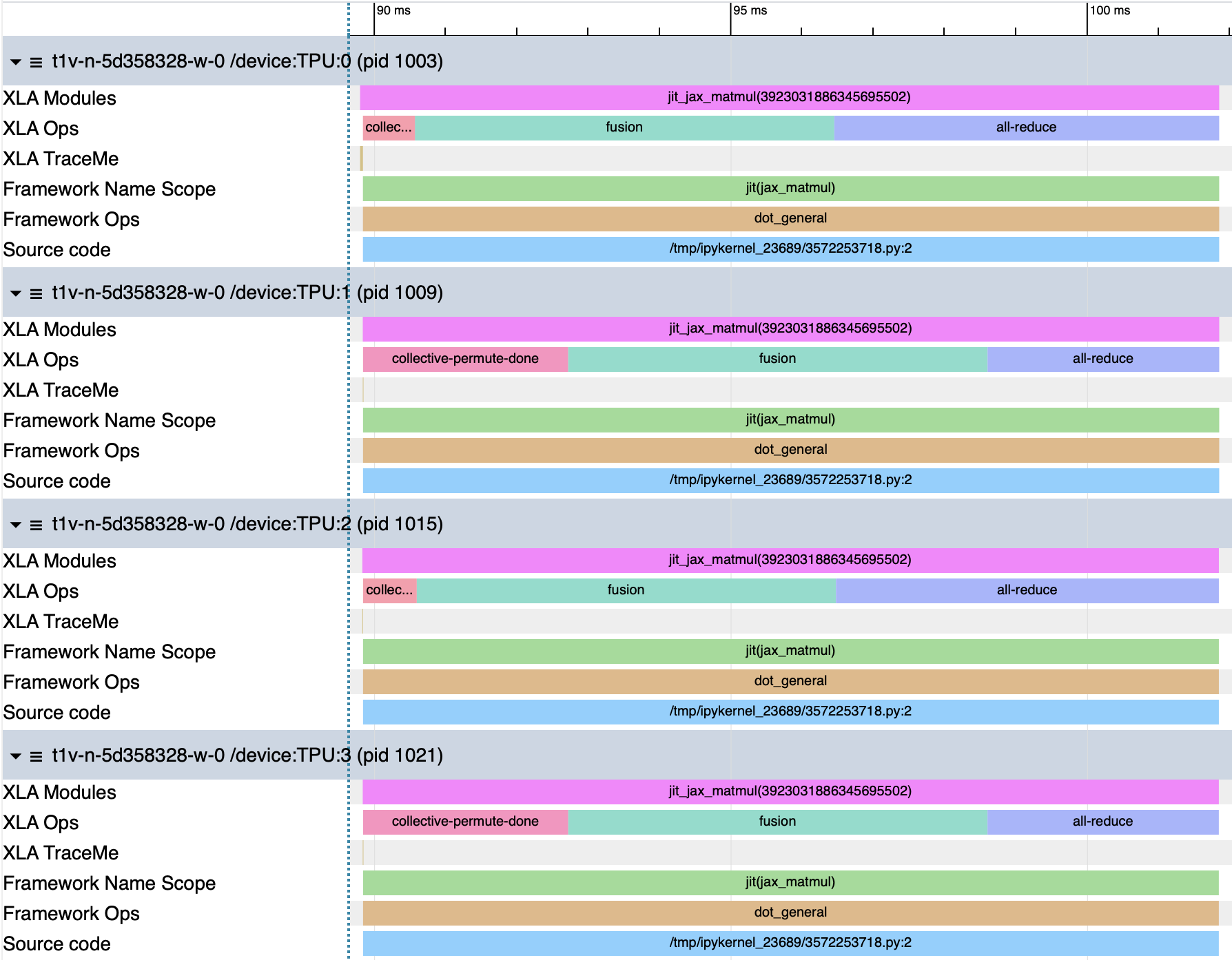
We begin with a simple Jax matmul as a reference. The profile shows us that the GEMM has been lowered to three distinct phases: an initial collective-permute, a fused operation that represents our device-local GEMM, and an all-reduce.
| Program | Step | Duration |
|---|---|---|
| Jax MatMul | Total | 12.05ms |
| collective-permute (Devices 0/2) | ~731us | |
| collective-permute (Devices 1/3) | 2.877ms | |
| fusion | 5.881ms | |
| all-reduce (Devices 0/2) | 5.4ms | |
| all-reduce (Devices 1/3) | 3.25ms |
Of our 12.05ms runtime, each device spends 5.88ms in the fusion operation. TPUv5e can achieve 197TFLOP/s, so from (2MNK / 4) / 0.005881 = 186.96TFLOPs we reach 95% of peak. The utilization is good when the MXUs are active, but the full operation only spends 49% of its time in compute. The shape of our profiles are suggestive. Devices 0 and 2 only spend 731us in the initial permute, while Devices 1/3 spend 2.877ms in that same permute. We can use the program’s HLO to help us understand how XLA structured the operation.HLO Dump
HloModule jit_jax_matmul,
is_scheduled=true,
entry_computation_layout={(bf16[8192,8192]{1,0:T(8,128)(2,1)}, bf16[8192,8192]{1,0:T(8,128)(2,1)})->bf16[8192,8192]{1,0:T(8,128)(2,1)}},
allow_spmd_sharding_propagation_to_parameters={false,false},
allow_spmd_sharding_propagation_to_output={true},
num_partitions=4

%add.clone (lhs.3: bf16[], rhs.3: bf16[]) -> bf16[] {
  %rhs.3 = bf16[]{:T(256)} parameter(1)
  %lhs.3 = bf16[]{:T(256)} parameter(0)
  ROOT %add.1 = bf16[]{:T(256)} add(%lhs.3, %rhs.3), backend_config={"flag_configs":[],"scoped_memory_configs":[],"used_scoped_memory_configs":[],"aliasing_operands":{"lists":[]}}
}

%bitcast_fusion (bitcast_input: bf16[8192,8192]) -> bf16[8192,8192] {
  %bitcast_input = bf16[8192,8192]{1,0:T(8,128)(2,1)} parameter(0)
  ROOT %bitcast = bf16[8192,8192]{1,0:T(8,128)(2,1)} bitcast(%bitcast_input)
}

%bitcast_fusion.1 (bitcast_input.1: bf16[8192,8192]) -> bf16[8192,8192] {
  %bitcast_input.1 = bf16[8192,8192]{1,0:T(8,128)(2,1)} parameter(0)
  ROOT %bitcast.1 = bf16[8192,8192]{1,0:T(8,128)(2,1)} bitcast(%bitcast_input.1)
}

%fused_computation (param_0: bf16[8192,8192], param_1: bf16[8192,8192]) -> bf16[8192,8192] {
  %param_0 = bf16[8192,8192]{1,0:T(8,128)(2,1)} parameter(0)
  %fusion.1 = bf16[8192,8192]{1,0:T(8,128)(2,1)} fusion(%param_0), kind=kLoop, calls=%bitcast_fusion
  %param_1 = bf16[8192,8192]{1,0:T(8,128)(2,1)} parameter(1)
  %fusion.2 = bf16[8192,8192]{1,0:T(8,128)(2,1)} fusion(%param_1), kind=kLoop, calls=%bitcast_fusion.1
  ROOT %convolution.1 = bf16[8192,8192]{1,0:T(8,128)(2,1)} convolution(%fusion.1, %fusion.2), dim_labels=bf_io->bf, metadata={op_name="jit(jax_matmul)/dot_general" stack_frame_id=10}
}

ENTRY %main.0_spmd (param: bf16[8192,8192], param.1: bf16[8192,8192]) -> bf16[8192,8192] {
  %param.1 = bf16[8192,8192]{1,0:T(8,128)(2,1)} parameter(1), sharding={devices=[2,1,2]<=[4] last_tile_dim_replicate}, metadata={op_name="rhs"}
  %param = bf16[8192,8192]{1,0:T(8,128)(2,1)} parameter(0), sharding={devices=[2,2]<=[4]}, metadata={op_name="lhs"}
  %collective-permute-start = (bf16[8192,8192]{1,0:T(8,128)(2,1)}, bf16[8192,8192]{1,0:T(8,128)(2,1)}, u32[]{:S(2)}, u32[]{:S(2)}) collective-permute-start(%param.1), channel_id=1, source_target_pairs={{0,0},{1,2},{2,1},{3,3}}, metadata={op_name="jit(jax_matmul)/dot_general" stack_frame_id=10}, backend_config={"flag_configs":[],"barrier_config":{"barrier_type":"CUSTOM","id":"1"},"scoped_memory_configs":[],"used_scoped_memory_configs":[]}
  %collective-permute-done = bf16[8192,8192]{1,0:T(8,128)(2,1)} collective-permute-done(%collective-permute-start), metadata={op_name="jit(jax_matmul)/dot_general" stack_frame_id=10}
  %fusion = bf16[8192,8192]{1,0:T(8,128)(2,1)} fusion(%param, %collective-permute-done), kind=kOutput, calls=%fused_computation, metadata={op_name="jit(jax_matmul)/dot_general" stack_frame_id=10}, backend_config={"flag_configs":[],"window_config":{"kernel_window_bounds":["64","8"],"output_window_bounds":["128","8"],"input_window_bounds":["128","4"],"estimated_cycles":"9557312","iteration_bounds":["8","8","16"],"cost_model_type":"COST_MODEL_TYPE_CLASSIC","ml_estimated_microseconds":0,"is_mask":false,"pad_output_on_minor_dim":"0","pad_input_on_minor_dim":"0"},"scoped_memory_configs":[],"used_scoped_memory_configs":[{"memory_space":"1","offset":"0","size":"13500416"}],"retry_config":{"retry_count":"0"},"convolution_algorithm_config":{"emitter":"EmitAllBatchInSublanes"},"aliasing_operands":{"lists":[]}}
  ROOT %all-reduce = bf16[8192,8192]{1,0:T(8,128)(2,1)} all-reduce(%fusion), channel_id=2, replica_groups=[2,2]<=[4], use_global_device_ids=true, to_apply=%add.clone, metadata={op_name="jit(jax_matmul)/dot_general" stack_frame_id=10}, backend_config={"flag_configs":[],"barrier_config":{"barrier_type":"CUSTOM","id":"0"},"scoped_memory_configs":[{"memory_space":"0","offset":"0","size":"67108864"}],"collective_algorithm_config":{"emitter":"RotatedPincerEmitter","strategy":"UniDirection1DRingStrategy","debug":"\nUniDirection1DRingStrategy{colors:2 phases:1 cores:{2},{2} nophase0:0 reserved_sflags:0 cross_module_on_2d_plane:0 has_reordering_map:0 use_routing_table_indices:0}"},"used_scoped_memory_configs":[{"memory_space":"1","offset":"0","size":"15532032"}],"retry_config":{"retry_count":"0"},"aliasing_operands":{"lists":[{"indices":["0","1"]}]}}
}
The sharding annotations on the parameters confirm our partitioning scheme:
param   -> sharding={devices=[2,2]<=[4]}
param.1 -> sharding={devices=[2,1,2]<=[4] last_tile_dim_replicate}
Our lhs, param, is sharded 2-way on both dimensions across our mesh. Our rhs, param.1, is sharded [2,1,2] with last_tile_dim_replicate, indicating that the second dimension is replicated along the second mesh axis. XLA handles this with a collective-permute.
%collective-permute-start = ...
collective-permute-start(%param.1),
source_target_pairs={{0,0},{1,2},{2,1},{3,3}},
...
Since on-diagonal devices have matching shards along the contracting dimension, for this topology and partitioning strategy, Devices 0/2 send data to themselves. The pairs {1,2} and {2,1} mean partitions 1 and 2 swap their y shards. That is Devices 1 and 3 exchanging data across the mesh while Devices 0/2 send to themselves. This exchange happens over the ICI links that connect TPUs into a mesh. After the collective-permute, every device has the y partition that aligns with its local x partition. TPUv5e has stated bidirectional ICI bandwidth of 45GB/s, so we expect sending 2x128 MiB over ICI to take ~2.98ms. The profiled transfer completes in 2.877ms, within ~0.1ms of the theoretical estimate.
After the local GEMM, an all-reduce sums partial results accumulated on each device:
replica_groups=[2,2]<=[4]
strategy: UniDirection1DRingStrategy
emitter: RotatedPincerEmitter
The strategy and emitter logic live in libtpu so the implementations are opaque, but XLA reserves 64 MiB of HBM and 14.81 MiB of VMEM for the all-reduce’s working buffers. The HBM reservation is half the size of the anticipated output array, so a simple ring-style communication pattern suggests each device is sending half its local, unreduced data over ICI and claiming the other half as its responsibility for the reduction. Sending 2x64 MiB bi-directionally uses the full 90GB/s ICI bandwidth, so the transfer time should cost 1.49ms comms latency to populate the receiving HBM buffers.
After the reduction, the same amount of data will need to be sent over ICI so that each device will have the full output, adding another 1.49ms to our all-reduce time. That yields a theoretical comms time of 2.98ms. The faster all-reduce phases complete in 3.25ms, while the slower phases trail by 2.15ms. This gap is consistent with each device’s exit timing from the collective-permute. The on-diagonal devices enter the all-reduce earlier and stall waiting for the off-diagonal devices to catch up.
Modeling the transfers this way leaves us with 0.27ms budgeted to perform the reduction. Data needs to be sent from HBM to VMEM to complete the reduction in between the send phases. Reading 64 MiB * 2 operands and writing 64 MiB with 810 GB/s HBM bandwidth should take 192 MiB / 810 GB/s = .249ms, leaving 0.021ms for the reductions. Reducing two [8192, 8192] matrices takes ~67.1MFLOPs, which implies ~3.2TFLOPs of VPU compute. While this VPU utilization is within this stated range, it’s possible that XLA is instead chunking the ICI transfers into smaller blocks to hide HBM and compute latency behind comms. We cannot glean the exact transfer pattern and sizes without the implementation, but the mechanics outlined above provide us the shape of operation.
XLA inserted a targeted collective-permute of the rhs shards, exchanging a minimal amount of data to align the contracting dimensions before entering the fusion. The devices that self-send can begin their computation immediately, so a bubble forms in the all-reduce portion of the profile waiting for those devices to catch up. Let’s try to replicate this behavior with Pallas. It is not strictly necessary to drop into LLO. These are the final VLIW bundles that compilation produces, not runtime measurements. LLO dumps help us understand the TPU’s internal ILP and scheduling decisions, but they are typically overkill for diagnosing kernel performance. There is relevant prior art in [6] and [7] if you’re interested in the compiler perspective. The LLO here is from the same matrix multiplication, but run on a single device. The Cloud TPU VM I was using reported the following error when I attempted to dump the full LLO compilation: Older versions of Jax + libtpu on Colab smoothed over this. It’s possible to AOT compile JAX programs for TPU without a device attached, though note that jaxlib requires AVX support. The GEMM fusion fans out to 115 distinct instruction types over 10,117 VLIW bundles. The structure is a software pipeline comprised of a prologue, a 3,200 step steady-state loop over 25 M-tiles * 8 N-tiles * 16 K-slices, and an epilogue. Each step advances three phases at once: prefetch the next tile from HBM into VMEM, compute the current tile on the MXUs, drain older results back to HBM. Work is distributed evenly across all four MXUs: The compiler round-robins across MXUs so pushes to MXU0/1/2/3 are interwoven with loads, pops, and vector accumulation. While one lane’s systolic pipeline is advancing, the scheduler uses neighboring bundles to issue work for other lanes. Below the staggered scheduling is visible across lanes. Each MXU sees 64 vmatpush.msra and 64 vmatpush.msrb instructions across the full kernel schedule, both derived from operand1 (rhs). That is 128 pushes per lane against 656 matmuls, or ~5 matmuls per push. Operand1 is staged into resident MXU bank slots and reused across multiple multiplies, while operand0 (lhs) is never pushed into bank state. Instead, it streams through the explicit vmatmul argument path, appearing as the gmra operand on all 2,624 matmuls. The volume of VPU work around the MXUs shows how much coordination is required to keep the MXU path hot. Of the 5,536 bundles containing MXU ops, 1,769 contain VMEM ops and 1,666 contain vector-side ops. The average bundle carries ~2.3 operations while the densest carries 12. Rhs flows through 1,024 loads, 512 pack/merge ops, and then 256 msra pushes plus 256 msrb pushes. Lhs flows through 656 direct loads, 1,995 spill-backed reloads, 328 pack ops, and then appears as the explicit gmra argument on all 2,624 matmuls. The results flow through the accumulator path, which sees 1,968 reloads, 658 mask/select ops, 5,248 pops, 5,248 adds, and 1,312 stores. The DMA descriptors in the LLO encode the geometry directly. The steady-state loop revisits two dma.hbm_to_vmem sites, one dma.vmem_to_hbm site, and three dma.done.wait sites. The field element_size_in_bytes: 2048 tells us one DMA element is an 8x128 bf16 layout block (8 * 128 * 2B = 2,048B), window_bounds says how many layout blocks to move, and size_in_granules measures the transfer in 32B units (one layout block = 64 granules). The stride triple (src, dst, steps) tells the DMA engine how to walk those blocks between the wide matrix layout in HBM and the compact tile layout in VMEM. On writeback the direction reverses, so the source and destination strides flip. The lhs and output windows are 82 * 8 = 656 rows by 8 * 128 = 1024 columns, while the rhs window is 1024x1024. The 656 rows are 82 layout row-groups of 8 rows each. The lhs matrix has 16,384 / 8 = 2048 total row-groups, but 25 tiles of height 82 require 2050, overshooting by 2 row-groups, or 16 rows. That is what pad_high is accounting for. The kernel uses 24 full M-tiles of 656 rows and one tail tile of 640 real rows plus 16 padded rows. The first prefetch appears at bundle 56, and the final writeback at bundle 10,093, so most of the schedule is spent in steady-state compute, with DMA priming at the front and drain at the back.An LLO Detour
F0303 05:37:58.574267 14193 llo_dumper.cc:471] Check failed: file::GetContents(path, &contents, file::Defaults()) is OK (NOT_FOUND: open failed for /home/reed/g3 /platforms/xla/service/jellyfish/tool_data/vmem_report_header.tmpl: No such file or directory
Op Per MXU Total vmatmul 656 2,624 vmatpush 128 512 vpop.f32.mrf 1,312 5,248 Category Count VMEM I/O (vld/vst/vstv) 7,582 Vector-side support (vadd, vsel, vor, vpack, etc.) 7,073 MXU drain (vpop.f32.mrf) 5,248 MXU matmul (vmatmul) 2,624 MXU feed (vmatpush) 512 DMA Descriptors
# LHS prefetch
0x37: dma.hbm_to_vmem /*src_stride=*/8192, /*dst_stride=*/512, /*steps_per_stride=*/32
    base_bounds: (2048, 128)
    dynamic_base_bounds: (2048, 128)
    window_bounds: (82, 8)
    iteration_bounds: (8, 25, 16)
    pad_low: (0, 0)
    pad_high: (2, 0)
    element_size_in_bytes: 2048

# Output writeback
0x276c: dma.vmem_to_hbm /*src_stride=*/512, /*dst_stride=*/4096, /*steps_per_stride=*/32
    base_bounds: (2048, 64)
    dynamic_base_bounds: (2048, 64)
    window_bounds: (82, 8)
    iteration_bounds: (8, 25, 16)
    pad_low: (0, 0)
    pad_high: (2, 0)
    element_size_in_bytes: 2048
Site Window Pad High Stride (src, dst, steps) LHS prefetch (82, 8) (2, 0) (8192, 512, 32) RHS prefetch (128, 8) (0, 0) (4096, 512, 32) O writeback (82, 8) (2, 0) (512, 4096, 32)
Adding a GEMM
If you would like to tinker with any of these kernels, note that you’ll need access to TPUs because 2D DMAs are not supported currently in interpret mode. The below diagrams are meant to be motivating not binding. The specific memory spaces and data movement will be dictated by the internal mechanics of the kernels that you write, so treat them as such.Jax Collectives + Pallas GEMM Kernel
def jax_pallas_gemm(lhs, rhs):
  rhs_full = jax.lax.all_gather(rhs, 'x', axis=0, tiled=True)
  this_y = jax.lax.axis_index('y')
  y_len = jax.lax.axis_size('y')
  k, n = rhs_full.shape
  k_block = k // y_len

  w_slice = jax.lax.dynamic_slice(rhs_full, (this_y * k_block, 0), (k_block, n))
  # Our kernel entry point is the make_matmul function
  local_out = make_matmul(lhs, w_slice, bm=512, bk=1024, bn=1024)
  return jax.lax.psum(local_out, 'y')
We’ll start by first allowing XLA to manage collectives, but swapping in a Pallas kernel for the GEMM computation. This implementation performs a full all-gather along the mesh x-axis so that the rhs matrix is replicated on each device. Because the lhs is still sharded over y, we have to suture in a dynamic slice to correctly pluck out the corresponding GEMM-local data. After the local computation completes, we insert an all-reduce over y to unreduce the shards.

The GEMM reference implementation is surprisingly compact at 11 lines of kernel code and a 15 line enclosing function. The two primary mechanisms to highlight are the grid and the block specs, which jointly let us control the software pipeline. The grid defines a nested loop that we traverse in lexicographic order, and the block specs are windowing functions. These windowing functions are not inert declarations. There is some argument dependent nuance, but when you supply an index map they are memory reservations and a DMA schedule, not lazy accessors. Before the kernel body runs, the compiler allocates a VMEM buffer of that shape for each input and output and DMAs the first window of data into it. Between grid iterations, the next window is DMA’d in and overlapped with compute via double buffering. Even if your kernel only touches a small slice of the data, the full block shape is allocated upfront. When you opt in to pipelining, the compiler hands you a slice and says here’s your data, do your thing.
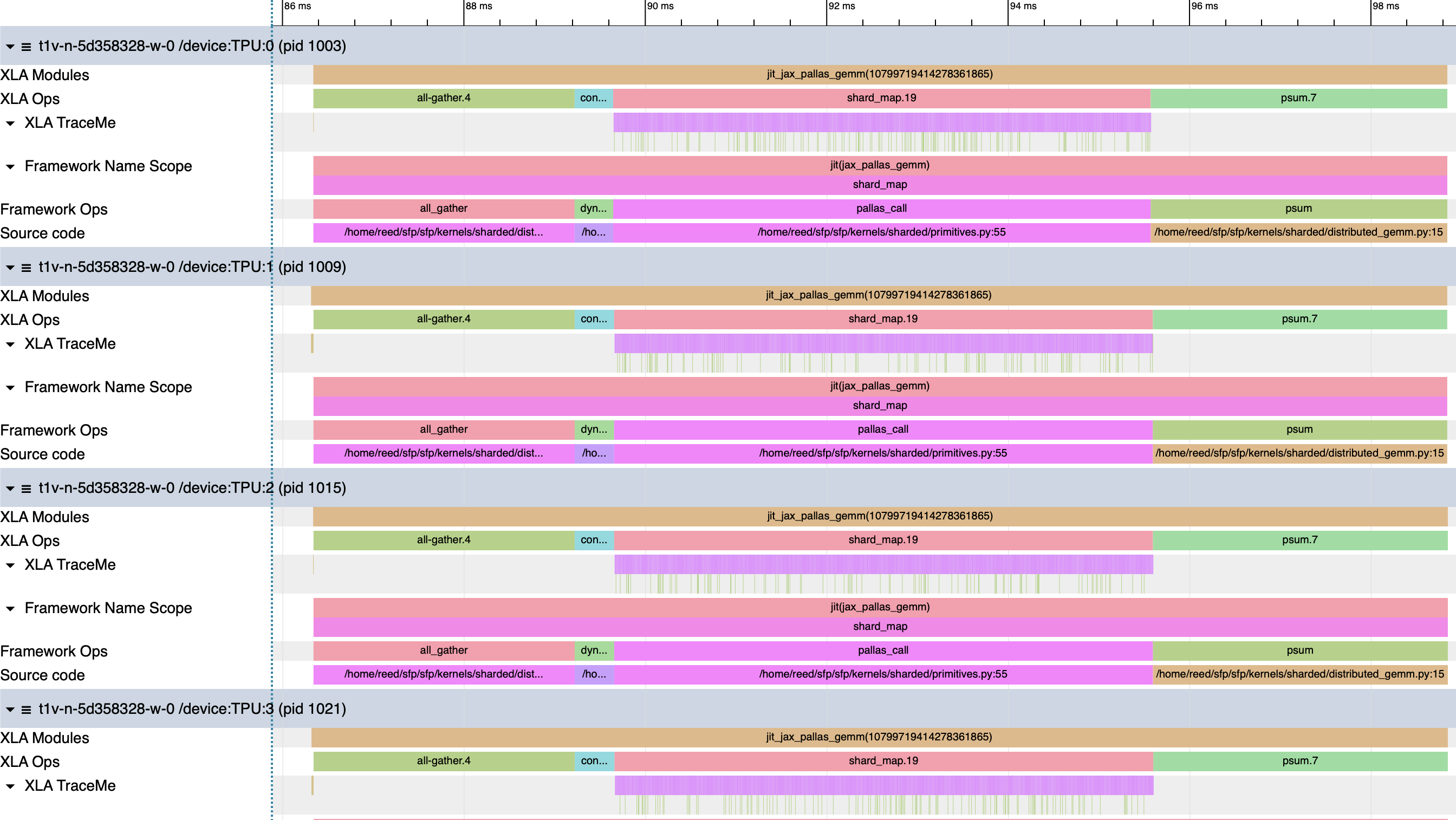
Annotating the kernel code liberally with jax.named_scope and compiling it with xla_enable_transpose_trace enabled [8], we get the following profile.
| Program | Step | Duration |
|---|---|---|
| Jax + Pallas Gemm | Total | 12.5ms |
| All-gather (XLA) | ~2.88ms | |
| Dynamic slice fusion | ~430us | |
| Pallas GEMM (shard_map.19) | ~5.93ms | |
| — compute GEMM | ~5.59us | |
| — zero scratch | ~348ns | |
| — flush to HBM | ~174ns | |
| psum / all-reduce (XLA) | ~3.25ms |
Each phase is fully serialized. Comparing the collective runtimes against the initial Jax implementation, the time spent in comms is equivalent, but we incur a 430us runtime penalty to slice the appropriate data out. We also send 2x more data because each device participates in the all-gather, adding 2x128 MiB ICI traffic.

The grid and block spec define traversal and access over our inputs and output. Blocked matrix multiplies lend themselves to spatial reasoning, so we define our grid points such that they range over the m/k/n dimensions of our operands. The grid encodes spatial information, and the block spec converts it into the appropriate addresses, plus buffer bookkeeping.
Let’s do some memory accounting to demonstrate the implicit buffering behavior. With bm=512, bk=1024, and bn=1024 tiles we have iteration bounds (16, 8, 8). Our inputs fetch blocks of lhs and rhs in (bm, bk) and (bk, bn) in bf16, and we reserve (bm, bn) tiles for our output. We also define an f32 accumulator of size (bm, bn) to store intermediates.
- LHS Tile: 512*1024*2 bytes = 1 MiB * 2 buffers = 2 MiB
- RHS Tile: 1024*1024*2 bytes = 2 MiB * 2 buffers = 4 MiB
- Output Tile: 512*1024*2 bytes = 1 MiB * 2 buffers = 2 MiB
- Accumulator: 512*1024*4 bytes = 2 MiB
That’s 10 MiB scratch space allocated in SRAM. The default scratch space capacity on TPUv5e is 16 MiB, so we have headroom to play with, though there is some small but real space set aside for register spills, semaphores, etc. If you have some Pallas kernels under your belt, you’re familiar with this error message: It tells us that our scratch space reservations are too large, and directs us to what looks to be Google internal documentation. Since Jax 0.8.2, we can call pltpu.get_tpu_info (or look here) to access device-specific properties. Our TPU has 128MiB of physical SRAM, but the compiler error tells us we fail above 16 MiB scoped VMEM. That limit appears to be a compiler-managed scoped working set, though without explicit documentation this is speculation. We can use a combination of xla flags and compiler params to increase our live scratch range. According to [17] “scoped_vmem can be tuned using xla_tpu_scoped_vmem_limit_kib. The hardware limitations for vmem are 64M for v5e, 128M for v6e, and 64M for v7x.”. The default scoped VMEM size of 16 MiB can be configured, but I haven’t rigorously tested when/if increasing this ceiling introduces subtles bugs or incorrectness.Dude where's my VMEM
> m, k, n = 16384, 16384, 8192
> # your code here
> result = matmul(x, y, bm=1024, bk=1024, bn=1024)
> result.block_until_ready()

JaxRuntimeError: RESOURCE_EXHAUSTED: Ran out of memory in memory space vmem while allocating on stack...
Scoped allocation with size 20.00M and limit 16.00M exceeded scoped vmem limit by 4.00M. It should not be possible to run out of scoped vmem -  see go/compile-time-vmem-oom#kernel-vmem-stack-oom for more information.
> pltpu.get_tpu_info()

TpuInfo(chip_version=<ChipVersion.TPU_V5E: 'v5e'>,
...,
vmem_capacity_bytes=134217728,
...
)
LIBTPU_INIT_ARGS="--xla_tpu_scoped_vmem_limit_kib=65536"
...
compiler_params=pltpu.CompilerParams(
    vmem_limit_bytes=24000000
)
Each iteration of our computation includes a tiled GEMM operation, and at the leading and trailing edges of our innermost dimension we have additional VPU traffic and an HBM write.
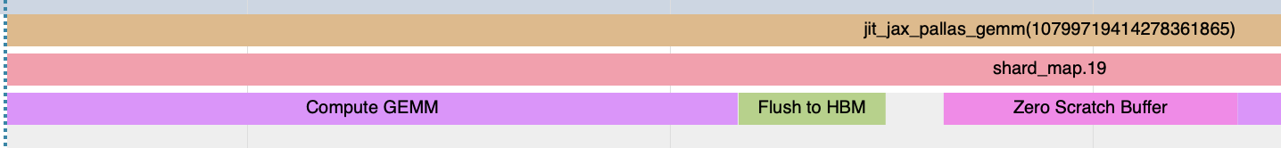 Inner Loop Boundary
Based on the numbers here, we can measure the kernel’s cycle efficiency. Our [8192, 8192] @ [8192, 8192] GEMM gets tiled into [512, 1024] @ [1024, 1024] subproblems that take ~5.593us each. Each subproblem requires 512*1024*1024 = 536M FMAs distributed over 4 MXUs, so 134M FMAs/MXU. At 16,384 FMAs/cycle/MXU with a 1.5 GHz clock, the theoretical minimum is 8,192 cycles or ~5.46us. Our measured time is 5.593us, ~8,390 cycles, which gives us 97.6% cycle efficiency.
At 5.593us/GEMM, we have 5.727ms of useful compute over the 5.93ms duration of the kernel. The profiled accumulator reset and HBM writes consume ~67us of our execution time, so they are marginal by comparison. But taking one last look at our flush to HBM, the profile consistently reports 174ns. Our accumulator is [512, 1024], and in bf16 that’s 1 MiB of data transferred over 810GB/s bandwidth HBM. That transfer should take ~1.29us. Our profiler appears to be reporting DMA enqueue time, not transfer time.
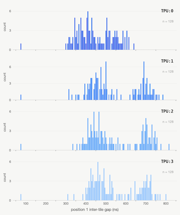 Gap timings between gemm 0 and gemm 1
When we inspect the profile closely we can detect contention between the enqueued write and the pipeline reads. This appears when we analyze sequential GEMMs. The gaps between GEMMs 2-7 are well-behaved at 70ns, but between the first GEMM, grid=(x, y, 0), and second GEMM, grid=(x, y, 1), of the innermost grid dimension, the time between GEMM stop/start has considerable jitter. The double buffering machinery and the accumulator write appear to be fighting for the memory controller’s attention. On this small example, the net effect of this jitter is negligible, but in it we see the processor’s shadow.
Compared to XLA’s native matmul, this approach is 3.7% slower. We don’t benefit from any of the compute/comms overlap because each stage is serial, and we’re paying an added formatting fee after the all-gather. We have compute wrapped in a kernel, so now we turn our attention to comms.
Do You Copy?
All Gather
The next step is to phase in hand-rolled communications, replacing XLA’s collective primitives with Pallas’s RDMA constructs. We’ll keep the same algorithmic shape from the previous example – all-gather over x, dynamic slice out the appropriate tiles, compute a GEMM, then reduce over y – but now each phase is a kernel we write and control.

all_gather_kernel_1D
def all_gather_kernel_1D(
  input_ref, output_ref,
  local_send_sem, send_sem, recv_sem,
):
  """
  input_ref: shard local data
  output_ref: out shard

  local_send_sem: allocates a semaphore for the local HBM copy
  send_sem: semaphore for the RDMA push
  recv_sem: semaphore for our local data
  """
  pid = pl.program_id(0)
  shard_height = input_ref.shape[0]

  # Get neighbors
  x_len = jax.lax.axis_size('x')
  this_x = jax.lax.axis_index('x')
  this_y = jax.lax.axis_index('y')
  right_device_x = jax.lax.rem(this_x + 1, x_len)

  # This is the _destination_ copy slot
  # Since we're moving things "right" along our mesh
  # We are forwarding whatever slice arrived from our left through the ring
  copy_slot_xright = jax.lax.rem(this_x - pid, x_len)

  # Self-send
  with jax.named_scope("Local HBM Copy"):
    @pl.when(pid == 0)
    def _copy_local_to_local():
      local_hbm_copy = pltpu.make_async_copy(
        src_ref=input_ref,
        dst_ref=output_ref.at[pl.ds(this_x * shard_height, shard_height), :],
        sem=local_send_sem
      )

      with jax.named_scope("Local Copy Start"):
        local_hbm_copy.start()
      with jax.named_scope("Local Copy Wait"):
        local_hbm_copy.wait()

  right_dma = pltpu.make_async_remote_copy(
    src_ref=output_ref.at[pl.ds(copy_slot_xright * shard_height, shard_height), :],
    dst_ref=output_ref.at[pl.ds(copy_slot_xright * shard_height, shard_height), :],
    send_sem=send_sem,
    recv_sem=recv_sem,
    device_id=(right_device_x, this_y),
    device_id_type=pltpu.DeviceIdType.MESH,
  )

  with jax.named_scope("Right DMA Start"):
    right_dma.start()
  with jax.named_scope("Right DMA Wait"):
    right_dma.wait()


def make_ag_1D(x):
  rows, cols = x.shape
  x_len = jax.lax.axis_size('x')

  grid_spec = pltpu.PrefetchScalarGridSpec(
    num_scalar_prefetch=0,
    # The pipeline for 2x2 mesh is one hop
    grid=(1,),
    in_specs=[
      # Our input reference is just a chunk in HBM
      pl.BlockSpec(memory_space=pl.ANY)
    ],
    # Our output reference will be another chunk in HBM
    out_specs=pl.BlockSpec(memory_space=pl.ANY),
    scratch_shapes=(
      [pltpu.SemaphoreType.DMA] * 2 # local_copy_op, send_sem
      + [pltpu.SemaphoreType.DMA] * 1 # These are our recv_sems. For 2x2, we only need 1 of them
    )
  )

  out_shape = jax.ShapeDtypeStruct((rows * x_len, cols), dtype=jnp.bfloat16)

  return pl.pallas_call(
    all_gather_kernel_1D,
    grid_spec=grid_spec,
    out_shape=out_shape
  )(x)
In the GEMM kernel, our grid represented a spatial traversal over data. By contrast, our all-gather doesn’t have data dependencies between grid points. The grid encodes ICI hops, or semantically time/steps. Each grid point is tracking the next exchange in a chain of forwarding operations.
For our 2x2 mesh, the x mesh ring has length 2, which means the all-gather completes in a single hop. Each device copies its local shard into the correct slot of the allocated output buffer with a local HBM-to-HBM copy, then fires an RDMA push to its neighbor along the x-axis. We use the device’s position in the ring and the current step to bulk forward the 128 MiB half of the matrix.
Our matrices never touch VMEM. The block specs use pl.ANY which disables the implicit pipeline machinery, instead handing us raw ref access into HBM. That means we take responsibility for that transfer with manual copies. This is the simplest possible use of the Pallas memory model. The kernel gets a handle to a region of HBM and we orchestrate DMAs against it directly.
All Reduce

all_reduce_kernel_1D
def all_reduce_kernel_1D(
    local_hbm_ref, output_ref,
    send_sem, recv_sem, copy_sem,
    local_scratch, recv_scratch
):
    y_len = jax.lax.axis_size('y')
    this_x = jax.lax.axis_index('x')
    this_y = jax.lax.axis_index('y')
    right_device_y = jax.lax.rem(this_y + 1, y_len)

    local_copy = pltpu.make_async_copy(
    src_ref=local_hbm_ref,
    dst_ref=local_scratch,
    sem=copy_sem
    )

    with jax.named_scope("Local Copy"):
        local_copy.start()
        local_copy.wait()

    send_ref = local_scratch
    for _ in range(y_len - 1):
        right_dma = pltpu.make_async_remote_copy(
            src_ref=send_ref,
            dst_ref=recv_scratch,
            send_sem=send_sem,
            recv_sem=recv_sem,
            device_id=(this_x, right_device_y),
            device_id_type=pltpu.DeviceIdType.MESH
        )

        with jax.named_scope("Right DMA Start"):
            right_dma.start()
        with jax.named_scope("Right DMA Wait"):
            right_dma.wait()

        with jax.named_scope("Add Remote Data to Local"):
            local_scratch[...] = local_scratch[...] + recv_scratch[...]

        with jax.named_scope("Write remote data to send slot"):
          send_ref = recv_scratch

    out_copy = pltpu.make_async_copy(
          src_ref=local_scratch,
          dst_ref=output_ref,
          sem=copy_sem
      )

    with jax.named_scope("Copy Out Start"):
        out_copy.start()
    with jax.named_scope("Copy Out Wait"):
        out_copy.wait()

def make_ar_1D(x, bm=1024, bn=1024):
    m, n = x.shape

    grid_spec = pltpu.PrefetchScalarGridSpec(
      num_scalar_prefetch=0,
      grid=(m // bm, n // bn),
      in_specs=[
          pl.BlockSpec((bm, bn), lambda i, j: (i, j)),
      ],
      out_specs=pl.BlockSpec((bm, bn), lambda i, j: (i, j)),
      scratch_shapes=(
          [pltpu.SemaphoreType.DMA] * 3 # send_sem, recv_sem, copy_sem
          + [pltpu.VMEM((bm, bn), jnp.bfloat16)] # local_scratch
          + [pltpu.VMEM((bm, bn), jnp.bfloat16)] # recv_scratch
          )
    )

    out_shape = jax.ShapeDtypeStruct(x.shape, x.dtype)

    return pl.pallas_call(
        all_reduce_kernel_1D,
        grid_spec=grid_spec,
        out_shape=out_shape,
    )(x)
The all-reduce kernel structure is different. The grid is spatial rather than sequential. The implied responsibility of each grid point is to reduce a chunk of data, not to forward data over the ring. The ring forwarding and accumulation logic lives inside the kernel body as an explicit loop. We tile our data into (bm, bn) blocks that fit in VMEM scratch, copy each block from HBM into a local scratch buffer, RDMA it along the y-ring, accumulate the received tile, and write back. The VMEM-to-VMEM DMAs over ICI mean we avoid the added tax of an HBM read on each hop.
The Pallas docs construct their all-reduce the other way around. Instead of a spatial grid with an inner loop over hops, they make the grid sequential. Each grid point is a ring step, and within each step you iterate over blocks of data. The algorithm is the same, but which dimension you hand to the grid machinery and which you manage yourself changes. The data tiling is spatial and naturally parallel. Each block can be reduced independently. The ring hops are sequential and inherently serial, with step two depending on the result of step one. We have to decide which one to promote to the grid and which one to absorb into the kernel body.
Serialized Kernel
Now that we have the individual phases of the original GEMM plucked out into kernels, let’s see how they perform.ag_gemm_ar_serial
def ag_gemm_ar_serial(lhs, rhs):
    this_y = jax.lax.axis_index('y')
    y_len = jax.lax.axis_size('y')
    ag = make_ag_1D(rhs)

    k_full, n = ag.shape
    k_block = k_full // y_len

    a_slice = jax.lax.dynamic_slice(ag, (this_y * k_block, 0), (k_block, n))
    gemm = make_matmul(lhs, a_slice, bm=512, bk=1024, bn=1024)
    return make_ar_1D(gemm)
| Program | Step | Duration |
|---|---|---|
| Serialized AG + GEMM + AR | Total | 13.17ms |
| shmap.19 — AG | ~3.32ms | |
| - Local HBM Copy | ~437.8us | |
| - DMA Wait | ~2.88ms | |
| Dynamic slice | ~415/439us | |
| shmap.20 — GEMM | ~5.93ms | |
| shmap.21 — AR | ~3.07ms | |
| - DMA Wait(s) | 45.47/46.5us | |
| - Add Remote Data to Local | ~1.085us | |
| copy.4 | ~408.7us |
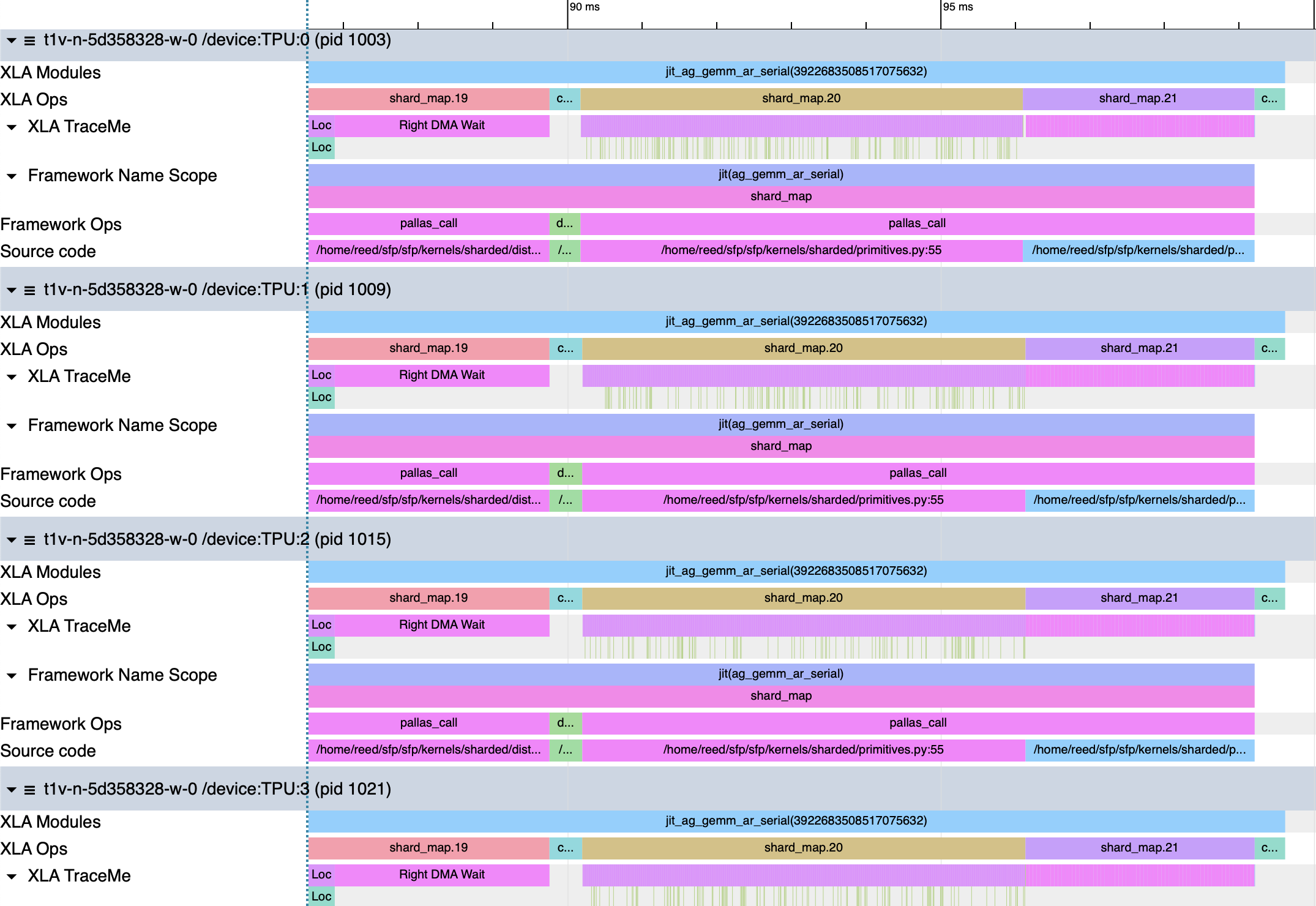
The kernel is broken up into five distinct blocks in the profile. There are 3 shard map calls that represent our individual kernels, the XLA dynamic slice, and a final copy operation after our all-reduce kernel exits. The GEMM execution time is the same as before, and all the reasoning that we did previously applies. We will focus our attention on the other blocks.
The total execution time of our function is 13.17ms, which is 9.3% slower than the reference implementation, and 5.4% worse than our GEMM-only kernel. In the all-gather there are two distinct phases of execution: one local copy operation, and one DMA operation. The local copy op is actually faster than the reference implementation’s collective-permutes at ~437.8us vs. 731us, though as we will see this is not without issue. The DMA that forwards data over ICI is 2.88ms, which is equivalent to XLA. The net difference here is that the RDMAs are blocked waiting for the local copy ops to complete. If instead we wrote the kernel to fire both operations asynchronously, we would reduce the execution time to max(t_local, t_dma) and recover 0.44ms of performance.
%constant_dynamic-slice_fusion = bf16[8192,8192]{1,0:T(8,128)(2,1)}
fusion(bf16[16384,8192]{1,0:T(8,128)(2,1)}
%shard_map.19, s32[]{:T(128)S(6)} %select_n.3),
kind=kLoop,
calls=%fused_computation
The dynamic slice adds a penalty to our runtime as it did in the GEMM-only kernel, and this penalty is not uniform across devices. Device 0 spends 414.6us in this operation, while the remaining devices spend 438.5us there. From the HLO we see that Jax’s select operation picks out a [8192, 8192] matrix from the fully replicated [16384, 8192] rhs data. The scalar device index from axis_index(‘y’) determines the slice offset. XLA lowers this to a kLoop fusion, meaning the program loops over our operand tile-by-tile to copy data to a new HBM allocation. On Device 0, dynamically evaluating the addresses needed for the copy seems to resolve to simpler index arithmetic. Devices 1-3 pay a ~34us penalty calculating dynamic values before copying them to a new allocation.
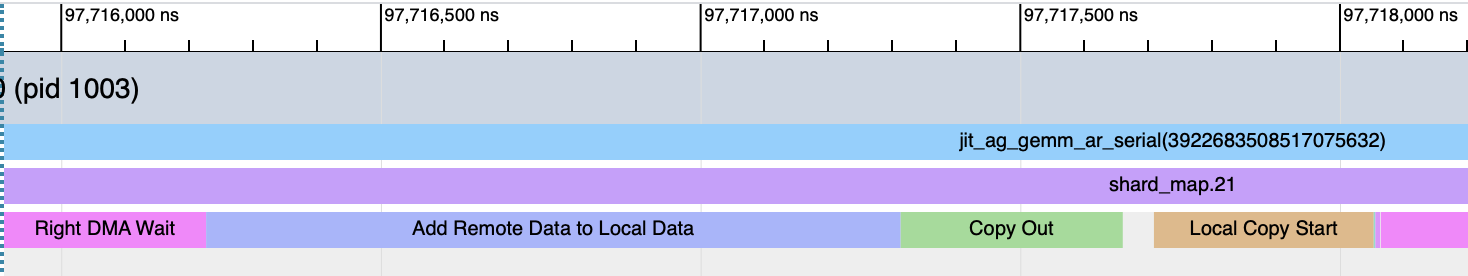
Our all-reduce is ~5.5% faster than the reference all-reduce. We lay [1024, 1024] tiles over our unreduced data, so the grid reduces to an (8,8) loop. Two scratch buffers are allocated to hold data from local HBM and to receive remote data from our neighboring device. Each iteration, we manually copy a tile from local HBM into VMEM, then launch an RDMA to exchange the current tile of data between devices. Once the data arrives, we add the buffers and manually write the data to our output HBM buffer. The shapes here were designed for perfect tiling, but this won’t always be the case. If your shapes produce partial tiles, you need to mask out the extra data to avoid subtle incorrectness bugs.
The 64 waits generated by the DMAs oscillate between ~46.5 and 45.47us. That’s 2 buffers*2 bytes*1024*1024 = 4 MiB sent simultaneously over ICI, which we expect to take 4 MiB/90 GB/s=~46.6us. The reductions themselves take 1.085us. That’s 1024*1024 FLOPs in 1.085us, or 966GFLOP/s. Though these seem like idealized conditions for the VPU because there is no MXU contention, this number is on the lower end of the stated VPU peak FLOPs range presented previously. That’s not to say we aren’t maxing the VPU out, just that we may need bigger problem sizes to evaluate the upper bound more precisely.
%copy.4 = bf16[8192,8192]{1,0:T(8,128)(2,1)} copy(bf16[8192,8192]{1,0:T(8,128)(2,1)}
%shard_map.21)
The epilogue copy following the all-reduce shard looks useless. The HLO shows us that the input and output are identical. We take the result of the all-reduce, and copy it into a new HBM buffer unchanged. The problem is that XLA cannot prove that it’s safe to reuse the all-reduce’s output buffer beyond the shard_map boundary. Pallas kernels get lowered through a separate IR, Mosaic, from regular Jax functions. Mosaic gets exposed to XLA as an opaque custom call. Because XLA can’t introspect the custom call, it has to be conservative about handling memory from these functions. XLA decides during its buffer assignment pass that it should copy the data to a new buffer rather than trying to use it in place. This defensive copy costs us 3.1% of our runtime for zero semantic work.
Introducing individual kernels for each phase lost us performance, which is strange because our all-reduce became more efficient, and we have a clear path to comparable performance for the all-gather. As we try to stitch these pieces together, we have to cooperate with XLA or pay boundary taxes. If we can fuse our kernels, we should be able to mitigate the awkwardness of communicating with Pallas and XLA.
Decomposing Grids
We’ve now seen grids do two different jobs. The GEMM kernel and all-reduce kernel used spatial grids while the all-gather kernel used a sequential grid. Grid dimensions carry implicit promises about independence. When you hand a dimension to the grid, you’re telling the compiler that these points can be scheduled, pipelined, and potentially reordered. A spatial grid over (m, n) tiles is safe because each point touches its own chunk of data, with at most a reduction over an accumulator. Sequence dimensions don’t have that property. If consecutive steps depend on one another, that ordering has to be enforced explicitly through semaphores, barriers, or loop-carried state. The grid won’t enforce it for you.
So far this hasn’t been a problem. Each kernel did one thing, and the grid could be designed around that single concern. When we want to fuse across kernel boundaries, we have to determine how to handle conflicting dependencies. The naive approach would be to cram everything into a single (ring_steps, m_tiles, n_tiles, k_tiles) grid and schedule comms and compute together, but this is fragile. The comms dimensions carry happens-before dependencies that the grid doesn’t enforce, and the spatial dimensions want to be pipelined with double-buffered block specs that assume stable inputs. If data is arriving mid-kernel over ICI, the block spec’s implicit data availability contract breaks down.
 Nesting pipelines with emit_pipeline
Pallas’s emit_pipeline interface allows us to decouple grids so that one grid doesn’t need to manage all these dependencies. An outer kernel can own the sequential logic, and inside the kernel we can launch a separate spatial pipeline for the compute work. The outer kernel decides when to compute and the inner pipeline decides how. In our present topology this decomposition feels minor. As the topology grows, the ring depth increases, the number of pipeline stages multiplies, and the fusion decisions become more complex. Using emit_pipeline gives us a natural mechanism to express algorithmic flexibility.
Let’s fuse a kernel.
Putting it Together
We set out to implement a version of the Jax reference matmul in pure Pallas. From our examination of HLO, Jax achieves higher performance by overlapping the initial data exchange and computation. We want to hide the ICI latency of the all-gather behind MXU work rather than paying for it serially.Emit Pipeline
def _emit_gemm_pipeline(x_ref, w_ref, o_ref, *, bm, bk, bn):
    """
    Emit a tiled GEMM pipeline.
    All refs are HBM. emit_pipeline handles VMEM tiling + double-buffering.
    """
    m, k_dim = x_ref.shape
    _, n = w_ref.shape
    grid = (m // bm, n // bn, k_dim // bk)

    def body(x_vmem, w_vmem, o_vmem, accum):
        @pl.when(pl.program_id(2) == 0)
        def _():
            accum[...] = jnp.zeros_like(accum)

        accum[...] += jnp.dot(
            x_vmem[...], w_vmem[...],
            preferred_element_type=jnp.float32,
        )

        @pl.when(pl.program_id(2) == pl.num_programs(2) - 1)
        def _():
            o_vmem[...] = accum[...].astype(o_vmem.dtype)

    @functools.partial(pl.run_scoped, accum=pltpu.VMEM((bm, bn), jnp.float32))
    def _(accum):
        pltpu.emit_pipeline(
            functools.partial(body, accum=accum),
            grid=grid,
            in_specs=[
                pl.BlockSpec((bm, bk), lambda i, j, k: (i, k)),
                pl.BlockSpec((bk, bn), lambda i, j, k: (k, j)),
            ],
            out_specs=pl.BlockSpec((bm, bn), lambda i, j, k: (i, j)),
        )(x_ref, w_ref, o_ref)
The above emit_pipeline implementation is taken from [8]. Notice that it is nearly identical to the reference Pallas GEMM kernel. The kernel code defined in body is supplied to pltpu.emit_pipeline, which handles the buffer management and pipelining similarly to pallas_call. Our enclosing function takes two input refs, an output ref, some tiling parameters, and returns a pipeline. We use run_scoped as a companion mechanism for the accumulator scratch allocation. The lifetime of the accumulator is scoped to the function body, so you don’t need to thread scratch buffers through the outer grid spec. The inner pipeline is self-contained and doesn’t leak VMEM concerns into the outer kernel’s HBM-level orchestration.Fused AG+GEMM Kernel
# FUSED AG GEMM
def fused_ag_gemm_kernel(
    input_ref,          # HBM: inputs shard (m, k)
    weight_ref,         # HBM: weights shard (k, n)
    output_ref,         # HBM: GEMM output (m, n)
    recv_weight_ref,    # HBM: workspace for received weights (k, n)
    send_sem, recv_sem, # RDMA semaphores
):
    """
    Outer kernel manages weight exchange (RDMA along x-ring).
    Inner pipelines handle the tiled matmul.

    On half the devices (x_idx == y_idx) the local weights are
    already correct, so GEMM runs entirely overlapped with RDMA.
    On the other half (x_idx != y_idx) we wait for the remote
    chunk then compute
    """
    this_x = jax.lax.axis_index('x')
    this_y = jax.lax.axis_index('y')
    x_len = jax.lax.axis_size('x')
    right_neighbor = jax.lax.rem(this_x + 1, x_len)

    BM, BK, BN = 512, 1024, 1024

    # Each device sends its shard right and receives from its left neighbor
    rdma = pltpu.make_async_remote_copy(
        src_ref=weight_ref,
        dst_ref=recv_weight_ref,
        send_sem=send_sem,
        recv_sem=recv_sem,
        device_id=(right_neighbor, this_y),
        device_id_type=pltpu.DeviceIdType.MESH,
    )

    with jax.named_scope("Start weight exchange DMA"):
        rdma.start()

    # When x_idx == y_idx (on-diagonal), MXU busy while ICI transfers the weight shard we need.
    with jax.named_scope("On Diagonal GEMM"):
        @pl.when(this_x == this_y)
        def _on_diag_gemm():
            _emit_gemm_pipeline(input_ref, weight_ref, output_ref, bm=BM, bk=BK, bn=BN)

    with jax.named_scope("Wait for Weight Exchange"):
        rdma.wait()

    # Block off-diagonal until after RDMA complete
    with jax.named_scope("Off Diagonal GEMM"):
        @pl.when(this_x != this_y)
        def _():
            _emit_gemm_pipeline(input_ref, recv_weight_ref, output_ref, bm=BM, bk=BK, bn=BN)


def make_fused_ag_gemm(lhs, rhs):
    m, k = lhs.shape
    _, n = rhs.shape
    x_len = jax.lax.axis_size('x')

    grid_spec = pltpu.PrefetchScalarGridSpec(
        num_scalar_prefetch=0,
        grid=(x_len // 2,),
        in_specs=[
            pl.BlockSpec(memory_space=pl.ANY),  # inputs
            pl.BlockSpec(memory_space=pl.ANY),  # weights
        ],
        # Two outputs: real output + HBM workspace for received weights
        out_specs=[
            pl.BlockSpec(memory_space=pl.ANY),  # GEMM output
            pl.BlockSpec(memory_space=pl.ANY),  # recv weight buffer
        ],
        scratch_shapes=(
            [pltpu.SemaphoreType.DMA]  # send_sem
            + [pltpu.SemaphoreType.DMA] # recv_sem
        ),
    )

    out_shape = [
        jax.ShapeDtypeStruct((m, n), lhs.dtype),   # GEMM output
        jax.ShapeDtypeStruct((k, n), rhs.dtype),  # recv workspace
    ]

    results = pl.pallas_call(
        fused_ag_gemm_kernel,
        grid_spec=grid_spec,
        out_shape=out_shape,
    )(lhs, rhs)

    return results[0]  # discard the workspace

def fused_ag_gemm_ar(lhs, rhs):
    partial = make_fused_ag_gemm(lhs, rhs)
    return make_ar_1D(partial)
| Program | Step | Duration |
|---|---|---|
| Fused AG + GEMM | Total | 12.3ms |
| DMA Wait | ~2.877ms | |
| On-diagonal GEMM | ~6.15ms | |
| Off-diagonal GEMM | ~5.96ms | |
| All-reduce (serial) | ~3.064ms | |
| On-Diagonal Stall | ~2.688ms | |
| copy.4 | ~408.9us |
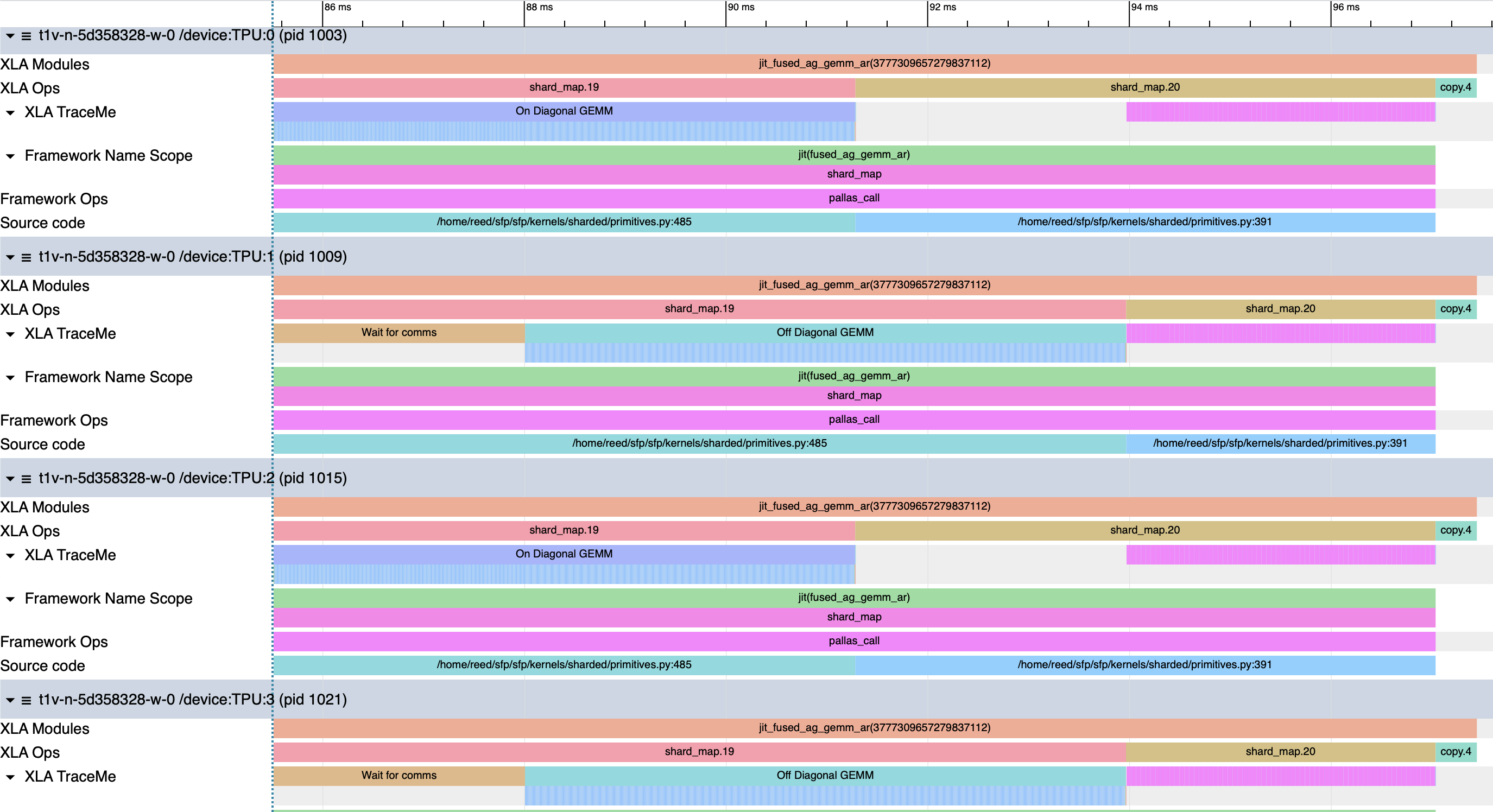
We can exploit this small topology directly. The kernel fires a single RDMA push of each device’s rhs shard to its neighbor along the x-ring. Two pl.when conditionals branch on device mesh location, expressed as x_idx==y_idx. On-diagonal devices immediately launch a full GEMM via emit_pipeline against their local weights while the RDMA is in flight. Off-diagonal devices have the wrong shard and must block on the receive semaphore until the exchange lands. The outer kernel body runs steps over a (x_mesh // 2) grid that owns the sequential structure, and we insert independent spatial pipelines when the data is available on each device.
We achieve the same oscillating pattern in our profile as the reference implementation. On-diagonal devices overlap ~6.15ms GEMMs with the ~2.877ms RDMA transfer while off-diagonal devices sit idle for that entire RDMA wait. Once the transfer completes, the off-diagonal devices execute a ~5.96ms GEMM, and the on-diagonal devices exit the kernel but stall before entering the all-reduce. The result is a bubble on each side. That’s 5.58ms of bubble time in a 12.3ms program. Nearly half the runtime is one side waiting for the other. The all-reduce adds another 3.06ms on top, and the straggler copy op remains.
This kernel is ~2.1% slower than the reference implementation. We’ve managed to recover the shape of the computation, but we’re being penalized in two distinct places, bubbles notwithstanding. If we found a way to tell XLA that the defensive copy after the all-reduce was unnecessary, our kernel runtime would drop to 11.91ms and we’d actually be ~1.2% faster. We also lose .197ms, 1.6% of our runtime, during the on-diagonal GEMMs compared to the off-diagonal GEMMs.
 Emit pipeline profile track
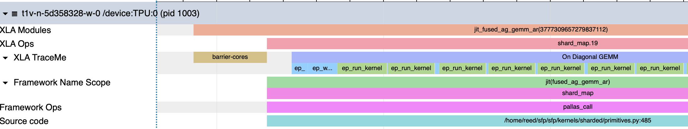
The pipeline emitter provides rich trace information that we can use to investigate this slow down. Each copy, wait, and GEMM execution is captured. All the device local GEMMs, marked ep_run_kernel, take the familiar ~5.595us, so we turn our attention instead to the waits.
| Wait Latency Percentile | On-diagonal (TPU:0) | Off-diagonal (TPU:1) |
|---|---|---|
| p50 | 7.5 ns | 7.5 ns |
| p90 | 416 ns | 8.7 ns |
| p99 | 1,870 ns | 440 ns |
| max | 3,535 ns | 2,575 ns |
Picking Devices 0 and 1 as our representatives, the on-diagonal wait latency distribution is heavily right-tailed. Though the medians are the same, Device 0 suffers significantly longer waits. Each device runs the same program, so GEMM kernels will have an identical number of waits. Plotting the latencies over the indices helps us to see what’s going on.
 Pipeline wait latency
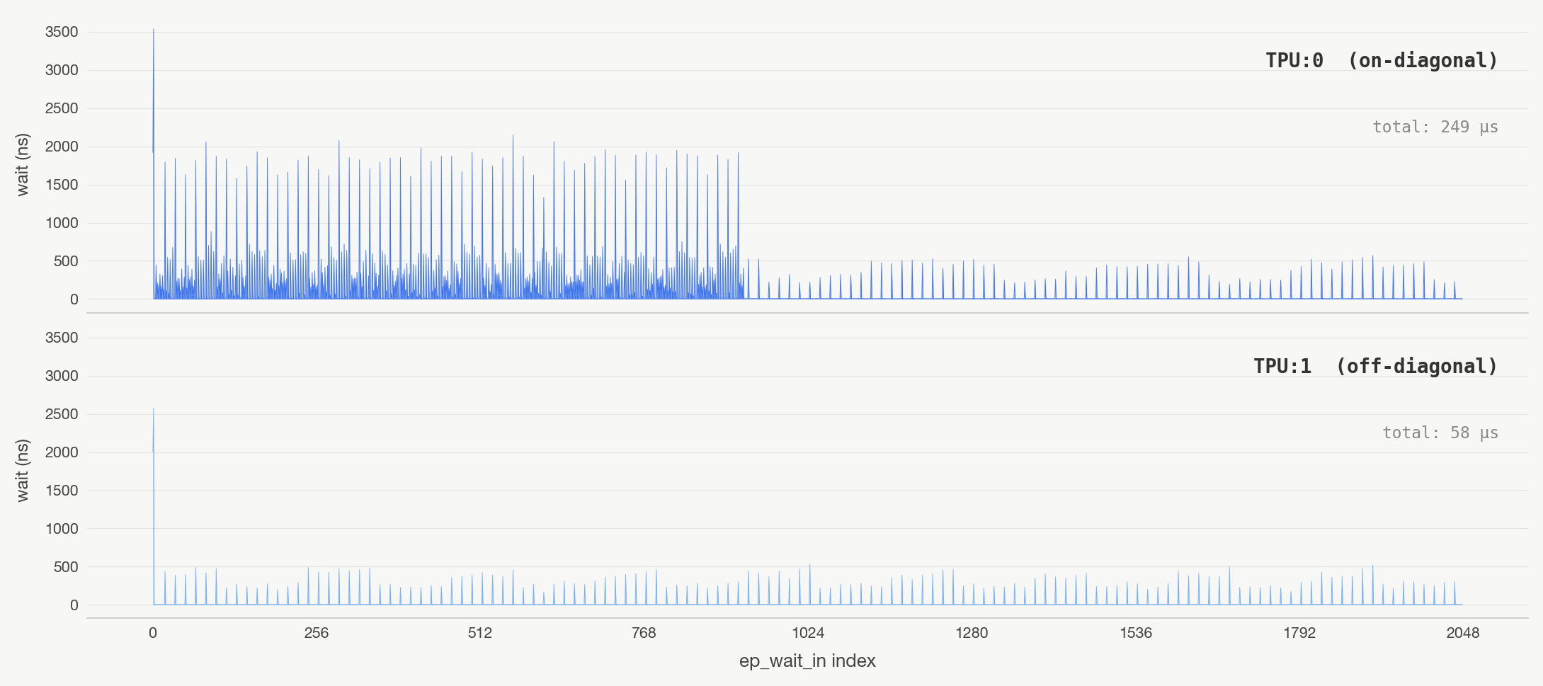
During the initial bubble, the on-diagonal pipelines are active while the device sends data over ICI. The compute and comms phases overlap for 924 calls to ep_wait_in. There is a marked difference before and after. It appears that the memory controller has to arbitrate between requests to device-local HBM and data arriving over ICI, pushing the wait latencies upwards.
| TPU:0 during comms | TPU:0 after comms | TPU:1 baseline | |
|---|---|---|---|
| median | 7.5 ns | 7.5 ns | 7.5 ns |
| p90 | 606 ns | 8.7 ns | 8.7 ns |
| max | 3,535 ns | 573 ns | 2,575 ns |
| total | 216 µs | 33 µs | 58 µs |
Once the exchange finishes, the prefetches have full bandwidth and the stalls disappear. Our on-diagonal GEMMs incur 191us of slowness, ~1.54% of our runtime performance, relative to our off-diagonal devices because of bandwidth contention.
When we scale to larger topologies, the details and the constraints begin to change. We’re forced to think more carefully about data hazards, runahead, ping-pong buffers, contended scratch space, bidirectional comms, turning GEMMs into GEMVs, and pipeline design for deeper computations. The pipeline bubbles get nastier, the resource contention gets worse, and the bugs become ever quieter. As an exercise, sketch out the grid you would use for the same partitions on a 4x4 mesh communicating unidirectionally, then bidirectionally.
Sand Castles
We haven’t painstakingly tuned everything that we could, but we aren’t here to squeeze every last ounce from this example. We’re here as ecologists. We needed to trudge through undergrowth and listen for footfalls to design kernels that parroted XLA. Arriving there allowed us to see a world of living puzzles. The remaining performance gains of the fused kernel aren’t from the implementation but a coordination cost with XLA. If we wanted, we could explore different DMA strategies, more granular transfers, different fusions, different tilings, and more. Those experiments are worth trying. The puzzles always lead to more puzzles. Scaling to larger topologies, or more complex kernels, requires rethinking how we sequence our pipelines over longer rings, more overlap stages, and less forgiving synchronization. Understanding the available moves on the board allows us to do that well in a gnarled game of 2048.
Pallas content is diffuse. It’s tribal knowledge hoarded in chests scattered in quiet alcoves. It’s visiting hamlets of thatch-roofed homes. It’s ambling in nomadic bliss collecting folk wisdom. When you finally return home with all that you’ve learned, all the meaning has dissolved back into indifferent, unflinching symbols. But as you scan them over and over, you start to notice their irregularities. Their meaning evolves and deepens, but they haven’t changed at all.
References
[1]: HTSYM – Distributed Computing in Pallas for TPUs
[2]: HTSYM – Rooflines
[3]: HTSYM – Sharded Matrices and How to Multiply Them
[4]: HTSYM – All the Transformer Math You Need to Know
[5]: How to Profile TPU Programs
[6]: From JAX to VLIW: Tracing a Computation Through the TPU Compiler Stack
[7]: When XLA Isn’t Enough: From Pallas to VLIW with Splash Attention on TPU
[8]: Pallas TPU: New and Advanced Features for Kernels | JAX/OpenXLA DevLab Fall 2025
[9]: Comp. Arch. - Lecture 27: VLIW Architectures (Fall 2025)
[10]: 6.S894: Accelerated Computing – Lab 11
[11]: Debugging Pallas
[12]: Optimizing NSA for TPUs - Kernel Worklog
[13]: SPMD in JAX #1: Sharding
[14]: MatText XLA Flags
[15]: Cloud TPU Performance Guide
[16]: XLA Flags Guidance
[17]: MaxText Benchmarking & Tuning Guide